Predictive Model for Housing Data
Scope:
Data analytics, predictive modeling, housing market and pricing strategies
Challenge & Goal:
The goal of the project was to extract publicly available housing data; assess price history and range against different variables like location, heating unit, number of bedrooms, and number of bathrooms; and find a correlation between the variables that predicts housing prices in urban areas.
The real estate and construction industry is not historically associated with data crunching and analysis. However, data analytics can play a significant role in profit-making in this industry. With help of data analytics, developers and real estate investors can predict the best areas and markets to invest and build their next developments. Research and consulting arms at real estate companies perform market intelligence and conduct a review of the past year’s housing data and trends as well as data-driven insight for potential real estate investing. Real estate companies can change their business models to adapt to a more revenue-generating format, and they offer wide variety of services to homebuyers and realtors. These services are not solely on the support side; they also include tools and insights for mitigating and transfering risk associated with large investments on properties. One of the biggest challenges for a real estate developer is to predict whether a housing development is worth investing in, due to the risk that the final price of the houses or the entire development might not be what the developer expected.
Approach:
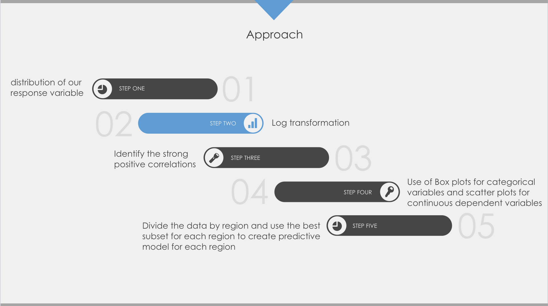
Our approach in developing the predictive model included a four-step process:
• The first step was initial research to identify which variables were significant for consideration as dependent variables. This step also involved identification of Variable type, namely Discrete and Continuous.
• The second step was to analyze the Discrete Variables and consolidate them into groups to reduce complexity of the model and at the same time retain the valuable information. This analysis also further reduced the number of variables.
• The third step was to analyze the Continuous Variables and eliminate any Continuous Variable if found insignificant.
• The fourth and final step was to insert the derived data obtained in the second step (now the new dependent variable). We eliminate all columns or fields that were no longer significant and used the reduced data set to create the predictive model.
Available Data
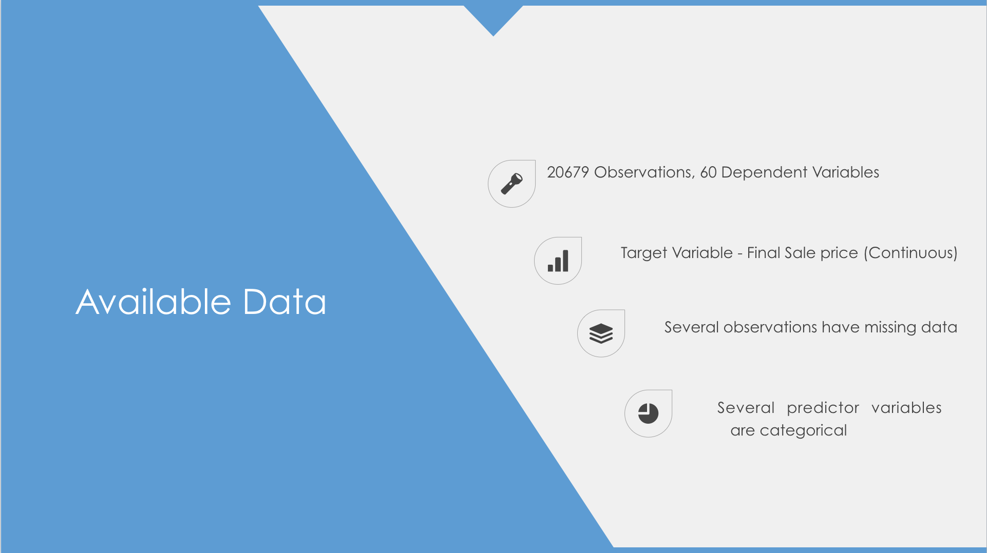
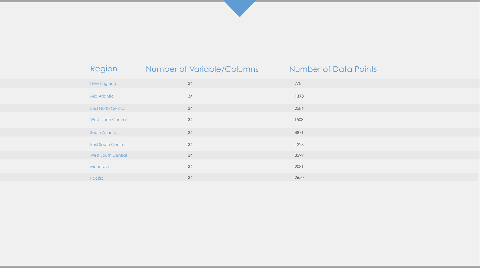
We were given two data sets, Training and Test. The Training data set was to be used for creating the Predictive Model and the Test Data set for application of the Predictive Model. The following table shows the details of the data available to us.
The target variable is ‘IsBadBuy’ which assumes a value of ‘0’ or ‘1’, to indicate whether it is a Bad Buy or not (1 for Bad Buy and 0 for Not a Bad Buy). Not all data is available for every data point, i.e. there are NULL values for some data points. Table 1 in Appendix shows the definition of each attribute of the available data and data issues if any. At this point we do not make any decisions about whether or not we use all the available variables for our predictive model. This happens in the subsequent steps.
Initial Data Analysis
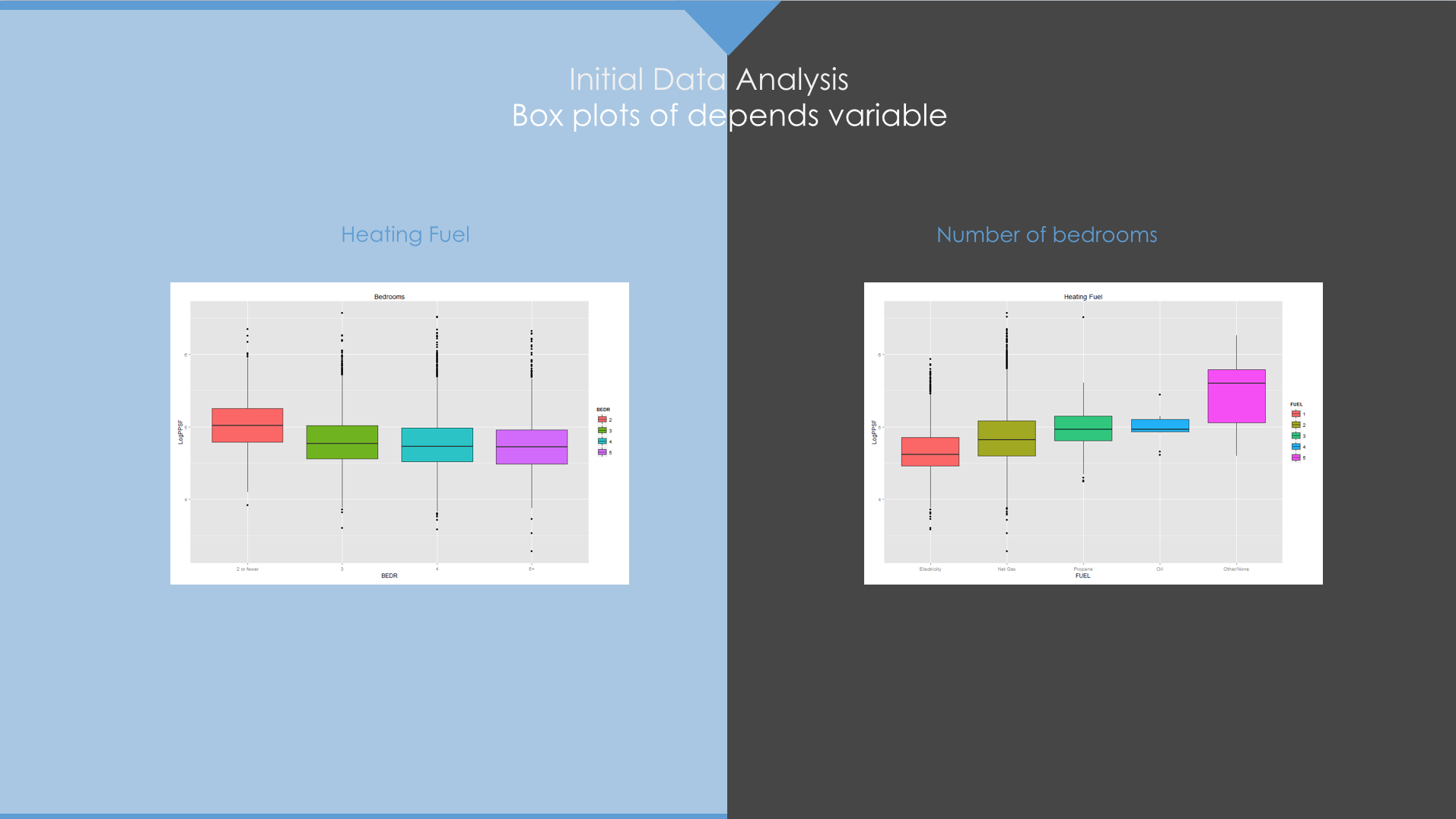
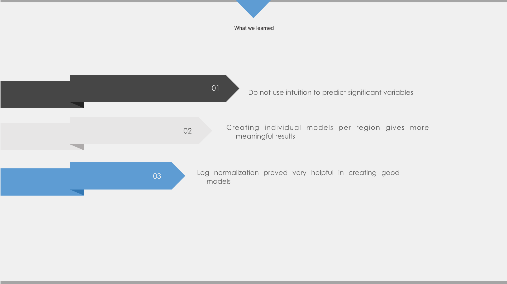
We analyzed all attributes/fields available and made use of some research to eliminate some of the dependent variables as candidates for our predictive model. Care was exercised not to eliminate any variable based only on intuition. In this step, we also identified variables that took discrete values, otherwise called Discrete Variables and Continuous Variables. These two variables were treated differently for Predictive Model analysis as seen in the subsequent sections.
Discrete Variables
From our Initial Data Analysis, we identified and marked all significant dependent variables as Discrete Variables and Continuous Variables. In this step, we further analyzed the Discrete Variables. As mentioned earlier, Discrete Variables are those variables that assume discrete values only, for example vehicle color, which assumes values like Silver, Red, White, etc. The objective of this step was to identify whether all the discrete variables that deemed significant in our initial analysis were truly significant or not. Once we found that a particular variable was significant, we then attempted to consolidate/group the discrete values. The value chosen to determine whether we could group discrete values together was Bad/Total Ratio. For example, if we were to find that all cars of colors Red, Blue and Green have Bad/Total Ratio within a 2% difference, we could group them together and create a new derived variable with name ‘Red or Blue or Green’. This consolidation helped reduce noise and simplify the model while retaining all information.
Discrete Variable Analysis and Consolidation
We further analyzed and consolidated the Discrete/Binary variables identified in the previous section. The first order of business was to check whether the variable had any significance at all, and if so, we could group the discrete values to reduce complexity while at the same time retaining all information. The detailed results of this analysis can be found in Discrete Variables section of Appendix. The following table shows the final result of this analysis. As the table makes clear, some of the variables that were considered significant or unresolved (TBD) were eliminated and the discrete values were grouped together.
Note: The consolidation of discrete variables into groups is based on the available data. If more data becomes available, this process should be repeated again as it may result in new groups or expansion of existing groups.
Continuous Variables
Unlike Discrete Variables, Continuous Variables assume continuous values, for example Vehicle Odometer. Also unlike Discrete Variables, it is not possible to group Continuous Variables. To determine whether or not a continuous variable is significant, we used box plots. In essence, we separated the data into two sets, one each for 0 and 1, that the target variable ‘IsBadBuy’ assumed, and observed how each box plot for these two sets appeared when each Continuous Variable was considered.
Collaborators: Vamsi Bhagavathula, Candice Richardson


